In this quick tutorial we will show you how to print gridlines in Microsoft Excel. These gridlines are the default separators or cell borders you see when you are working on an Excel spreadsheet. A lot of people don’t want to spend unnecessary time formatting borders and rows/column separators. This neat feature comes built in with Excel. However, it is surprising that not many people know about it.
We have made a video to show how to print gridlines and borders in your Excel spreadsheet. Below the video, you will also find step by step instructions with images.
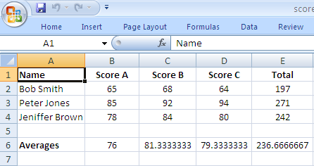
1. Open the spreadsheet or worksheet you want to print with gridlines or borders.
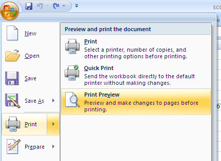
2. Go to “Print Preview”
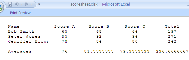
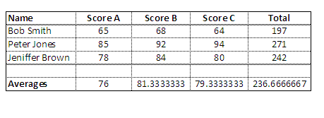
3. This is how your worksheet would look like in print preview.
4. Click on “Preview” and then click on “Page Setup”. This will open the page setup dialogue box.
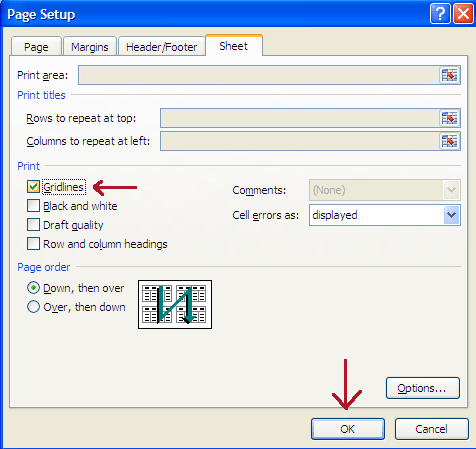
5. Go to the “Sheet” tab, check the “Gridlines” option and then click “Ok”.
6. Now your spreadsheet would look like this in the print preview.
You can now choose to print your spreadsheet or close the print preview.
In the default view, you will notice that your spreadsheet is as it is and no formatting has changed on it. But it will print with the gridlines when you send it to the printer.
Also note that if you want to print a sheet without gridlines you can always go to the Page Setup and uncheck the gridlines option.
Comment Summary
No summary generated.

Great effort and I like the nice and clear site you have. A few kins and errors here and there. But the video needs to be worked at. The sound is barely audible.